Tutorial 1a: Generating the Collision Matrices

---

Before any time evolution can be simulated, the effects of collisions between hard spheres must be pre-computed. This pre-computation is conducted by the functions contained within the DiplodocusCollisions sub-package of Diplodocus, which generate collision matrices that describe the rate at which some incoming state of spheres will be scattered into some outgoing state.

This process is required whenever you want to include a binary interaction in your simulation, that is any interaction that involves two incoming particles and two outgoing particles, e.g. two incoming spheres that collide to create two outgoing spheres.

Generating the Collision Matrices

Particle Names

First thing is to select the names of the four particles involved in the binary interaction $12\to 34$. In Diplodocus, each particle species is designated a unique three letter string to identify it. These unique identifiers are then used internally to define the properties of the particles (please refer to Particles, Grids and Units for more details). In binary interactions, we follow the convention that the pairs of names (12) and (34) should be in alphabetical order. Therefore for the interaction between hard spheres the names are declared as:

using Diplodocus

name1 = "Sph"
name2 = "Sph"
name3 = "Sph"
name4 = "Sph"

Momentum Space Grids

Next is to define how momentum space is to be discretised for each particle species. Given that spheres are the only species here, we only need to define the discretisation for them, this includes the upper and lower bounds of momentum magnitude $p$ (upper and lower bounds for polar angle cosine $u$ and azimuthal angle $h$ are not requrired as they are assume to be bounded by $[-1,1]$ and $[0,2\pi ]$), grid types (see Particles, Grids and Units) and the number of grid bins. These must be of the format p_low_name, p_low_name, p_grid_name, p_num_name, u_grid_name, u_num_name, h_grid_name and h_num_name where name is the abbreviated three letter name of the particle species.

For this tutorial we will select the momenta $p$ ranges from ${10}^{-5}{m}_{\text{Ele}}c$ to ${10}^4{m}_{\text{Ele}}c$ consisting of 72 bins, 9 uniformly sized bins in polar angle cosine and 1 uniformly sized bin in azimuthal angle (i.e. axisymmetric).

p_low_Sph = -5.0
p_up_Sph = 4.0
p_grid_Sph = "l"
p_num_Sph = 72

u_grid_Sph = "u"
u_num_Sph = 9

h_grid_Sph = "u"
h_num_Sph = 1

Monte-Carlo Setup

The elements of collision matrices are generated using a Monte-Carlo method as they are integrals of high dimension. We must define how many times each momentum bin is to be sampled by this Monte-Carlo approach. This is defined by three values: numLoss defines the number of incoming states (i.e. sets of $({\overrightarrow{p}}_1,{\overrightarrow{p}}_2)$ vectors, which in this case define the momentum vectors for the two incoming spheres about to collide) to sample per incoming state momentum bin, numGain defines the number of outgoing states (i.e. ${\overrightarrow{p}}_3$ and ${\overrightarrow{p}}_4)$, defining the momentum of the spheres after colliding) to sample for each outgoing state bin in momentum space, and numThreads defines the number of threads to use (see the documentation for multi-threading in Julia).

TIP

The larger numLoss and numGain are, the more accurate the integration will be, but this will take more time.

numLoss = 16
numGain = 16
numThreads = Threads.nthreads()

WARNING

By default this script uses the maximum number of available threads Threads.nthreads(), if you would prefer the scripts to run with fewer threads then modify the variable numThreads to the desired amount.

Further, to improve the Monte-Carlo sampling, we can deploy importance sampling by defining a non-zero scale factor. This scale factor weights the sampling of outgoing state towards the centre-of-momentum direction. Useful for high energy scatterings where particles are preferentially scattered towards that direction. As the user, you can set this scale factor to take a range of values a:b:c where a is its minimum value, b is the step size and c its maximum value (a multiple of b).

scale = 0.0:0.1:0.2

TIP

For the first round of integration it is advised to run with a scale of zero i.e. scale = 0.0:0.1:0.0 as weighting may not be needed for accurate integration. If inaccuracy is found, the scale should be increased gradually.

Where to Save the Collision Matrices

We now need to define where to store the generated collision matrices. This can be defined by specifying fileLocation as the path to the desired folder. If left unspecified, this location will default to joinpath(pwd(),"Data") i.e. a folder named Data found in the current directory. If the specified fileLocation does not exist, it will be created when this script is run.

fileLocation = joinpath(pwd(),"Data")

Final Setup and Running

We can bundle all the above user defined parameters into a tuple called Setup. This is generated by the UserBinaryParameters() function, which reads the above parameters from Main. It also generates the fileName under which the collision matrices will be saved and stored.

(Setup,fileName) = UserBinaryParameters()

WARNING

It is not advised to edit fileName as its format is used internally by DiplodocusCollisions and DiplodocusTransport to identify the appropriate collision matrices to load.

Finally, we can run the Monte-Carlo integration using the function BinaryInteractionIntegration:

BinaryInteractionIntegration(Setup)

TIP

Even on a good system, integration typically takes several hours if not days. But once it's done the matrices can be used over and over again. So don't worry, and while you wait perhaps sit back, relax and read that book that's been on your shelf for years just waiting to be read.

Checking the Collision Matrices

The evaluation of the collision matrices relies on Monte-Carlo sampling, therefore accuracy isn't guaranteed. There are several functions within Diplodocus aimed to assist with determining if the integration accuracy is sufficient for use.

Plotting the Spectra

The most visual approach is to use the plotting function InteractiveBinaryGainLossPlot from DiplodocusPlots. This creates an interactive plot in which the user can look at different incoming states and view the resulting outgoing spectra. To use this function, first load the file containing the collision matrices using BinaryFileLoad_Matrix:

Output = BinaryFileLoad_Matrix(fileLocation,fileName);
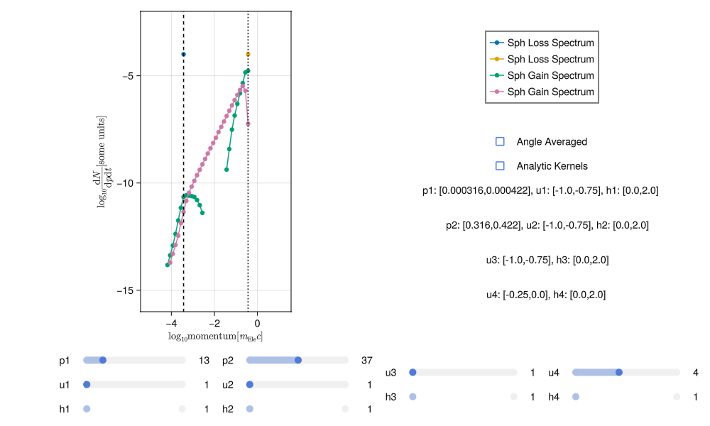
InteractiveBinaryGainLossPlot(Output)

This will display the plot in a separate window where you can interact with it. There are sliders for the the discrete bins of the two incoming particles momentum p1 and p2, and their propagation directions, in spherical polars u ($u=\cos \theta$) and h ($phi$). There are then also sliders for the outgoing particles directions with the spectra of outgoing states as a function of momentum being plotted.

As an example of poor integration, the plots below show a noisy spectra most likely due to insufficient sampling of incoming and outgoing states:

This noise can be reduced by increasing the number of points sampled in each momentum bin (i.e. running the integration again with more numLoss and numGain).

TIP

Re-running the integration with BinaryInteractionIntegration will re-use the previous integration to generate a more accurate result instead of starting again from scratch.

With sufficient sampling the spectra should have much less noise, something like this:

Generating good spectra involves a bit of trial and error. It is very easy to tell when a spectra is poor but it may take some practice to get used to how increasing the sampling and adjusting the scale affect the results.

TIP

If a specific range of incoming states seems to be particularly poorly sampled, you can focus on that regime by specifying the input parameters p1loc_low, p1loc_up, p2loc_low, p2loc_up, these can be set to any Int64 values that specify range of incoming momentum bins to sample from low to up. The integrator will then not sample incoming states from outside this region.

Another way to judge the accuracy of integration is through the DoesConserve function. This prints to the terminal a series of statistics about the integration. For the "good" integration this looks like:

DoesConserve(Output)

sumGainN3 = 43913.3488697066
sumGainN4 = 0.0
sumLossN1 = 45317.327934271074
sumLossN2 = 0.0
sumGainN = 43913.3488697066
sumLossN = 45317.327934271074
#
sumGainE3 = 1.3633630831974214e8
sumGainE4 = 0.0
sumLossE1 = 1.4088172759030634e8
sumLossE2 = 0.0
sumGainE = 1.3633630831974214e8
sumLossE = 1.4088172759030634e8
#
errN = -1403.9790645644753
errE = -4.5454192705641985e6
ratioN = 0.9690189353926422
ratioE = 0.9677359204184194
#
mean error in N = -0.013605041174533096
std of error in  N = 0.06949470100280596
#
mean error in E = -0.012232423226154596
std of error in E = 0.06954381657360521

It includes, the total gain and loss of particles as well as the total gain and loss of energy (note as all particles are identical the gain and loss of particles 2 and 4 are neglected as they are identical to 1 and 3). The ratio of particles and energy in and out ratioN and ratioE respectively should be around 1.0 for good integration. These values give a sense of overall convergence but also provided are statistics for individual incoming to outgoing states. For a single incoming state (one set of $p1,u1,h1,p2,u2,h2$ bins) an error in particle number and energy can be calculated by comparing the loss matrix element for that state to the sum of all outgoing gain matrix elements that correspond to that incoming state. mean error in N then gives the mean of that error and std of error in N gives the standard deviation. In the case here the mean error is around 1% with a standard deviation of around 6%.

Corrected Spectra

The above raw 1% error in particle number and 1% error in energy before and after a collision is not bad, but over many timesteps this will to poor conservation of number and energy.

There are two ways to improve this: first is to just increase the sampling by re-running the integration as described above. The second is to apply a correction to the outgoing spectra to enforce conservation of number and energy. This latter method guarantees conservation to numerical precision and is already built into DiplodocusCollisions. In brief, it applies two corrective scalings, one to the entire spectrum and one to the highest momentum bins. This ensures that the total gain of outgoing particles and their energy matches that of what is lost from the incoming states, which maintaining the shape of the spectra as much as possible.

This corrective step is applied as part of the integration and the resulting collision matrices can be accessed by setting corrected=true as an option of BinaryFileLoad_Matrix e.g.

Output = BinaryFileLoad_Matrix(fileLocation,fileName,corrected=true);
DoesConserve(Output)

sumGainN3 = 45317.32792698461
sumGainN4 = 0.0
sumLossN1 = 45317.32792987315
sumLossN2 = 0.0
sumGainN = 45317.32792698461
sumLossN = 45317.32792987315
#
sumGainE3 = 1.408817275737935e8
sumGainE4 = 0.0
sumLossE1 = 1.4088172758223104e8
sumLossE2 = 0.0
sumGainE = 1.408817275737935e8
sumLossE = 1.4088172758223104e8
#
errN = -2.8885406209155917e-6
errE = -0.008437544107437134
ratioN = 0.9999999999362597
ratioE = 0.999999999940109
#
mean error in N = 1.0081429301433313e-13
std of error in  N = 2.344515870818534e-11
#
mean error in E = 1.584577307280524e-11
std of error in E = 7.65965128057108e-11

Now the conservation statistics for particle number and energy are accurate to machine precision, allowing much longer simulations to be run without worrying about conservation issues.

Running such a simulation is what we will do next!